Once analytical data have been collected is a good practice to plot a frequency distribution – how many times each value occurs – or a histogram. The bars in the histogram show how many times each value occurred in the data set. The observed values are placed in the x-axis.
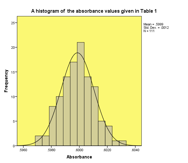
Let us consider as an example the absorbance values that we get by measuring a solution containing a substance A with known concentration c using a U.V./Visible spectrophotometer. The absorbance values are given in Table 1. A histogram of the absorbance values is shown in Figure 1.
 |
| Table 1: Absorbance values obtained by measuring a solution of substance A by a U.V/Visible spectrophotometer |
 |
| Fig. 1: A histogram of the absorbance values given in Table 1. The plot indicates a normal distribution (the curve shows the idealized shape of the normal distribution) |
Frequency distributions such as the one shown in Fig. 1 can be very useful for assessing properties of the distribution of the observed absorbance values such as:
- The tallest bar gives us the value that occurs more often. It is called the mode of the distribution.
- The shape of the distribution gives us information about the distribution of the data around the mode. For example in the distribution shown above the data are distributed symmetrically around the mode (if you draw a vertical line through the center of the distribution then it should look the same on both sides). This distribution is called a normal distribution and is characterized by the bell-shaped curve. This distribution shows that the majority of values lie around the center of the distribution – shown by the largest bars around the central value.
- If the distribution is not symmetrical around the center then it is called a skewed distribution. In a case like this frequent values are clustered at one end of the scale and the frequency of values falls of towards the other end (Fig. 2). Therefore, we get a positively or negatively skewed distribution.
- If the distribution shows pointiness (or kurtosis) - like the one in Fig.2 – then a lot of values are close to the center of the distribution and almost there are no values in the tails. This distribution is called leptokurtic. If the distribution has many values in the tails then shows a plateau at the center and is called platykurtic.
- In a normal distribution the values of skew and kurtosis are 0 (the distribution is neither too pointy or too flat and is perfectly symmetrical).
- The normal distribution of measurements is the fundamental starting point for analysis of data. It shows the mean of a large population of measurements x̅ (x̅ approaches μ for an infinite number of measurements, where μ is the true mean of the population). When a large number of measurements are made in order to determine the value of a physical or chemical quantity, the individual measurements are not all identical and equal to the accepted value x̅ , which is the mean of the infinite population, but are scattered about x̅, owing to random error. The normal distribution curve expresses the distribution of errors (x- x̅) about the true value μ ( and is also known as the error curve or probability curve). The term error curve arises when one considers the distribution of errors (x- x̅) about the true value μ.
- The breadth or spread of the curve indicates the precision of the measurements and is determined by and related to the standard deviation s.
- Frequency distributions (including the normal distribution) give us some idea of how likely a given value is to occur – what is the probability that a given value will occur. This is the reason they are also called probability distributions. A probability value can range from 0 (there is no chance the value would occur ) to 1 (the value definitely would occer). For example a 0.2 probability means that there is 20% chance that something will happen.
To explain this, let us suppose that we would like to find the probability that the absorbance value 0.6014 (Table 1) would occur assuming a normal distribution. From Table 1 we can see that this value actually occurred 2 times in 111 measurements (~ 1.8% chance to occur).
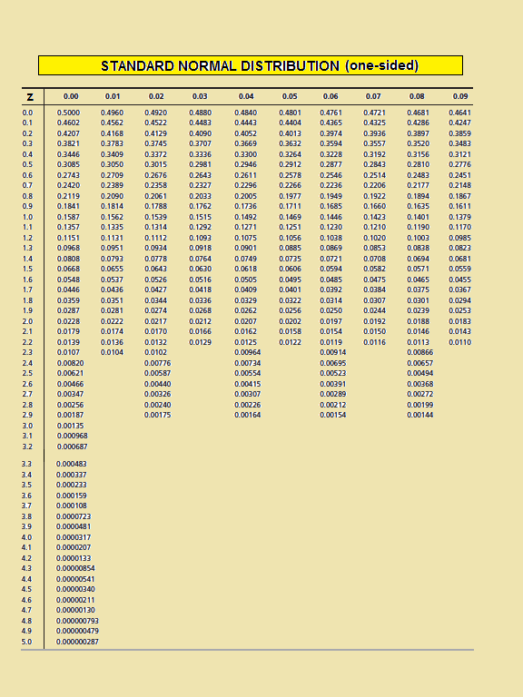
Suppose that we did not have Table 1. Then in order to calculate the above, we would use an idealized normal distribution with a mean value x̅ = 0 and a standard distribution s=1 that statisticians use to calculate the probability of getting particular values based on the frequencies with which a particular score occurred in the distribution (see Table 2: Standard Normal Distribution).
The obvious problem is that the absorbance data in Table 1 do not have a mean value x̅ = 0 and a standard distribution s=1 (as a matter of fact they have x̅ = 0.599 and a standard distribution s=0.0012, see Fig. 1). Therefore we have to convert the data so they have x̅ = 0 and a standard distribution s=1. In order to center the data at zero, we take each value x and subtract from it the mean of all values x̅. Then, we divide the resulting value by the standard deviation s to ensure that the data have a standard deviation of 1. The resulting scores are known as z-scores:
z = (x - x̅ )/ s (1)
where z a value of a normal distribution with x̅ = 0 and s = 1, x a value of a normal distribution, s the standard deviation of the distribution.
So by substituting x = 0.6014 in (1) we get: z = (x - x̅) / s = (0.6014 – 0.599) / 0.0012 = 1.25
From Table 2 (Table of the Standard Normal Distribution) we get that for z = 1.25 the probability is 0.10565 or 10.5% chance that a higher absorbance value than 0.6014 would occur. For the same z value the probability is 0.8943 (1-0.10565 = 0.8943) or 89,4% chance that a lower absorbance value than 0.6014 would occur.
 |
| Table 2: Standard Normal Distribution (one-sided) |
It is obvious from this example that the normal distribution and z-scores allows us to calculate the probability that a particular value will occur. This is very useful as it will be shown in due course.
Certain z-scores are particular important – because their values cut off certain important percentages of the distribution - such as:
i) z = +1.96 and z = -1.96 because these cut off the top and bottom 2.5% of the distribution respectively. Both of them together cut off 5% of the distribution or say it differently 95% of the z-scores lie between -1.96 and +1.96.
ii) z = +2.58 and z = -2.58 because these cut off together 1% of the distribution or say it differently 99% of the z-scores lie between -2.58 and +2.58.
iii) z = +3.29 and z = -3.29 because these cut off together 0.1% of the distribution or say it differently 99.9% of the z-scores lie between -3.29 and +3.29.
References
1 D. Harvey, “Modern Analytical Chemistry”, McGraw-Hill Companies Inc., 2000
2 R.D. Brown, “Introduction to Chemical Analysis”, McGraw-Hill Companies Inc.,
1982
3 A. Field, “Discovering Statistics using SPSS” , Sage Publications Ltd., 2005

Tidak ada komentar:
Posting Komentar